Analysis of community composition

Introduction

Plotting bar plots and ordinations from the highest transfer volume (1800 ul)

Libraries and global variables

library(tidyverse)
library(here)
library(fs)
library(fishualize)
library(Polychrome)
library(withr)
library(scales)
library(patchwork)

source(here::here("R", "utils_generic.R"))

data_raw <- here::here("_data_raw", "20240318_BTK_illumina_v3")

# make processed data directory if it doesn't exist
data <- here::here("data", "20240318_BTK_illumina_v3")
figs <- here::here("figs", "20240318_BTK_illumina_v3")

fs::dir_create(data)
fs::dir_create(figs)

Read data

counts <- read_tsv(here::here(data, "species_counts_md.tsv")) %>% 
  mutate(libprep = case_when(str_detect(sample, "_bp$") ~ "boil",
                             str_detect(sample, "_qg$") ~ "qiagen"))

counts_f <- counts %>% 
  group_by(sample) %>% 
  mutate(f=norm_count/sum(norm_count)) %>%  
  ungroup()

Processing/analysis

Check for failed samples

counts_f %>% 
  group_by(sample) %>% 
  summarize(sum = sum(count)) %>% 
  arrange(sum)

So there were a surprising number of qiagen samples that basically failed with very few reads. Not sure why this happened but regardless we will exclude samples with fewer than 500 reads for the next steps.

failedsamps <- counts_f %>% 
  group_by(sample) %>% 
  summarize(sum = sum(count)) %>% 
  arrange(sum) %>% 
  filter(sum < 500) %>% 
  pull(sample)

counts_f <- counts_f %>% 
  filter(sample %nin% failedsamps) %>% 
  mutate(mygroup = paste0("amp: ", amp_conc, " | evo: ", evo_hist, " | day = ", day, " | rep = ", replicate)) %>% 
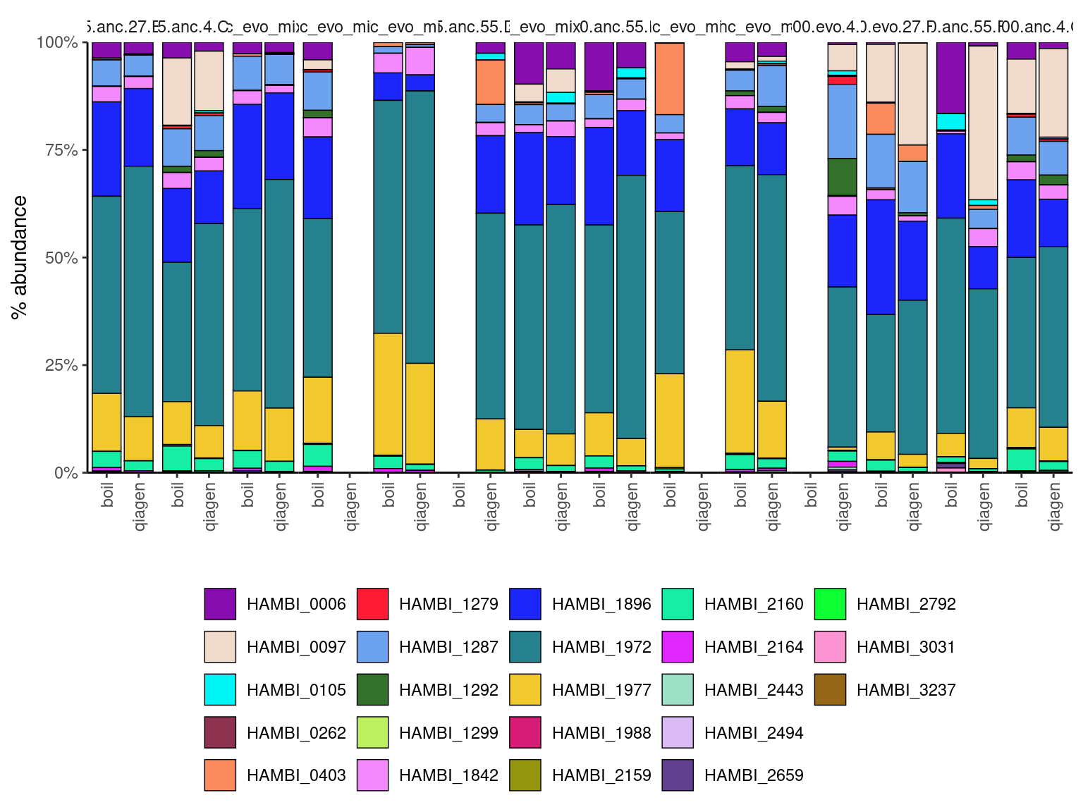
  mutate(mygroup = interaction(amp_conc, evo_hist, day, replicate))

Plot two extraction methods side by side ::: {#fig-01}

ggplot(counts_f) +
    geom_bar(aes(y = f, x = libprep, fill = strainID), 
             color="black",
             linewidth=0.25, 
             stat="identity",
             position = "stack") +
    facet_grid(~ mygroup, labeller = label_wrap_gen(width = 25)) +
    scale_fill_manual(values = hambi_colors) +
    scale_y_continuous(limits = c(0,1), expand = c(0, 0), labels = percent) +
    scale_x_discrete(guide = guide_axis(angle = 90)) +
    labs(x="", y="% abundance") + 
    theme_bw() +
    theme(
    panel.spacing.x = unit(0,"line"),
    strip.placement = 'outside',
    strip.background.x = element_blank(),
    panel.grid = element_blank(),
    panel.border = element_blank(),
    panel.background = element_blank(),
    axis.line.x = element_line(color = "black"),
    axis.line.y = element_line(color = "black"),
    legend.title = element_blank(),
    legend.background = element_blank(),
    legend.key = element_blank(),
    legend.position = "bottom"
    )

:::

Look in terms of absolute differences between boil and qiagen across all samples.

counts_f %>% 
  mutate(sample2 = str_extract(sample, ".+_\\d+")) %>%  
  dplyr::select(sample2, libprep, strainID, mygroup, f) %>% 
  pivot_wider(id_cols = c(sample2, strainID, mygroup), names_from = "libprep", values_from = "f") %>% 
  mutate(diff = qiagen - boil) %>%  
  ggplot() +
  geom_jitter(aes(x = strainID, y = diff, color = mygroup), width = 0.15) +
  scale_x_discrete(guide = guide_axis(angle = 90)) +
  scale_y_continuous(labels = percent) +
  scale_color_manual(values = rainbow(14, s=.6, v=.9)[sample(1:14,14)]) +
  labs(x = "", y = "Qiagen minus Boil (%)")

Warning: Removed 92 rows containing missing values or values outside the scale range
(`geom_point()`).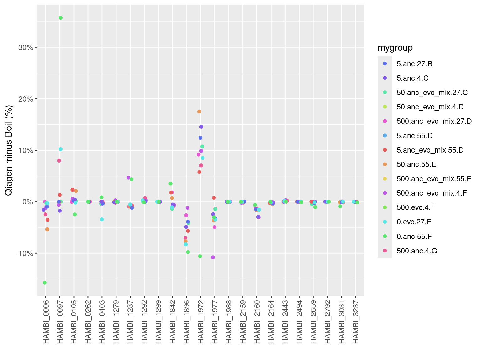

Figure 1

The deviations, again, look quite consistent meaning for each species the deviation seems to be in the same direction (positive/negative) and about the same magnitude. This would imply that we can correct for this using metacal…

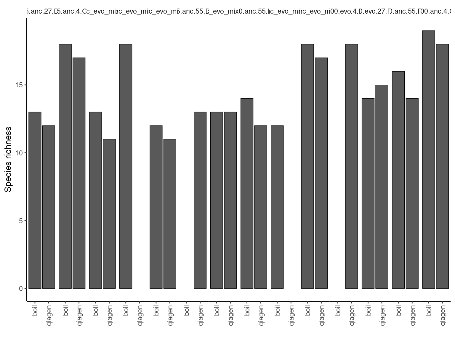
counts_f %>% 
  filter(f > 0) %>% 
  group_by(sample) %>% 
  summarize(richness = n_distinct(strainID)) %>% 
  ungroup() %>% 
  left_join(distinct(dplyr::select(counts_f, mygroup, sample, libprep, amp_conc, replicate, evo_hist, day))) %>% 
  ggplot() +
    geom_bar(aes(y = richness, x = libprep), 
             color="black",
             linewidth=0.25, 
             stat="identity",
             position = "stack") +
    facet_grid(~ mygroup, labeller = label_wrap_gen(width = 25)) +
    scale_x_discrete(guide = guide_axis(angle = 90)) +
    labs(x="", y="Species richness") + 
    theme_bw() +
    theme(
    panel.spacing.x = unit(0,"line"),
    strip.placement = 'outside',
    strip.background.x = element_blank(),
    panel.grid = element_blank(),
    panel.border = element_blank(),
    panel.background = element_blank(),
    axis.line.x = element_line(color = "black"),
    axis.line.y = element_line(color = "black"),
    legend.title = element_blank(),
    legend.background = element_blank(),
    legend.key = element_blank(),
    legend.position = "bottom"
    )

Joining with `by = join_by(sample)`