Analysis of community composition

Introduction

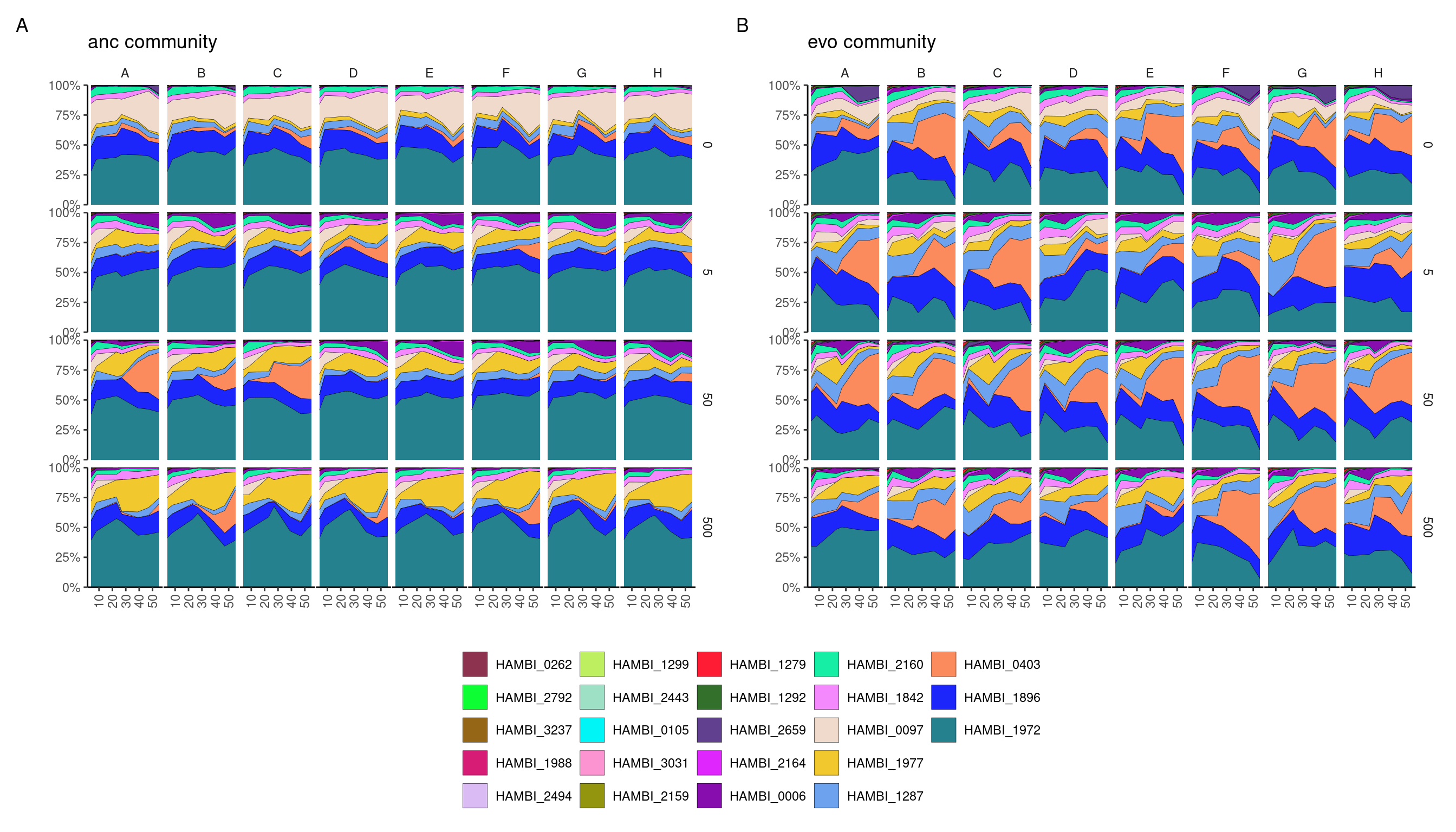
Area plots of community composition

Libraries and global variables

library(tidyverse)
library(here)
library(fs)
library(fishualize)
library(Polychrome)
library(withr)
library(scales)
library(patchwork)

source(here::here("R", "utils_generic.R"))

data_raw <- here::here("_data_raw", "20240513_BTK_illumina_v3")

# make processed data directory if it doesn't exist
data <- here::here("data", "20240513_BTK_illumina_v3")
figs <- here::here("figs", "20240513_BTK_illumina_v3")

fs::dir_create(data)
fs::dir_create(figs)

Read data

counts <- read_tsv(here::here(data, "species_counts_md.tsv")) %>% 
  rename(evo_code = evolution) %>% 
  mutate(evolution = case_when(evo_code == "E2" ~ "evo",
                               evo_code == "E3" ~ "anc"))

Helps make the area plots look nicer

strain.order <- counts %>% 
  group_by(strainID) %>% 
  summarize(m = mean(f)) %>% 
  arrange(m) %>% 
  pull(strainID)

Plot community compositions from the experiment

phi <- counts %>% 
  mutate(strainID=factor(strainID, levels=strain.order)) %>% 
  group_by(evolution) %>% 
  group_split() %>% 
  map(myarplot) %>% 
  wrap_plots(., ncol = 2) +
  plot_layout(guides = 'collect') +
  plot_annotation(tag_levels = 'A') & 
  theme(legend.position = 'bottom')

Warning: Using `size` aesthetic for lines was deprecated in ggplot2 3.4.0.
ℹ Please use `linewidth` instead.

phi

Figure 1: Temporal trajectories of community composition during the experiment. Columns in the grid show experimental replicate, while rows in the grid show the experimental applied ampicillin concentration in \(\mathrm{\mu g/ml}\).